
Monte Carlo Analysis is used in financial planning software to estimate the risk that an investment portfolio misses its goal. In goals-based financial planning, this is the top concern. Will a financial plan fail by running out of money? Monte Carlo analysis introduces randomness to a plan to see how it affects the outcome. The analysis runs multiple trials of your financial plan, holding some inputs constant while allowing others to randomly change to see how the financial plan is affected. In most financial planning software, the variable factors are the investment returns in any given year. Investment returns are volatile, and so it makes sense to see how the financial plan's outcome is affected by random investment returns. Running Monte Carlo simulations allow us to see risks that may not be apparent otherwise.

If we assume a random return from investments in each year and run the simulation enough times, we can answer some important questions about the financial plan, including:
- What is the likelihood of success for the financial plan? This helps us understand whether the financial plan is on track. Too low of a success rate could mean you need to contribute more to your accounts, lower the amount of your after-tax goal, or delay the start date of your after-tax goal. Too high of a success rate means you may end the plan with too much money left.
- In the scenarios that failed, what was the median year of failure? This may give us additional comfort. For example, let us suppose that your financial plan is for retirement and your after-tax goal lasts from the time you are 65 until 95. If your plan's Success Rate is 75% and fails 25% of the time, it means that the failed iterations ran out of money before the age of 95. This could be concerning. However, if those failed plans ran out of money at an median age of 94, you may be somewhat comforted.
The constants in the financial plan include the starting balances of the accounts assigned to the plan, account contributions, the after-tax goal, the starting date of the after-tax goal, how many years the after-tax goal is needed, and any income that could be used to satisfy the after-tax goal. You can read more about these inputs in our article on Financial Planning.
This remainder of this article focuses on the random variable - investment returns, and also addresses how some other financial planning software fall short.
The Random Variable: Investment Returns
We need to estimate three key factors about an investment to determine the probability of an investment's return in any given year:
- Arithmetic return
- Standard deviation
- Distribution shape
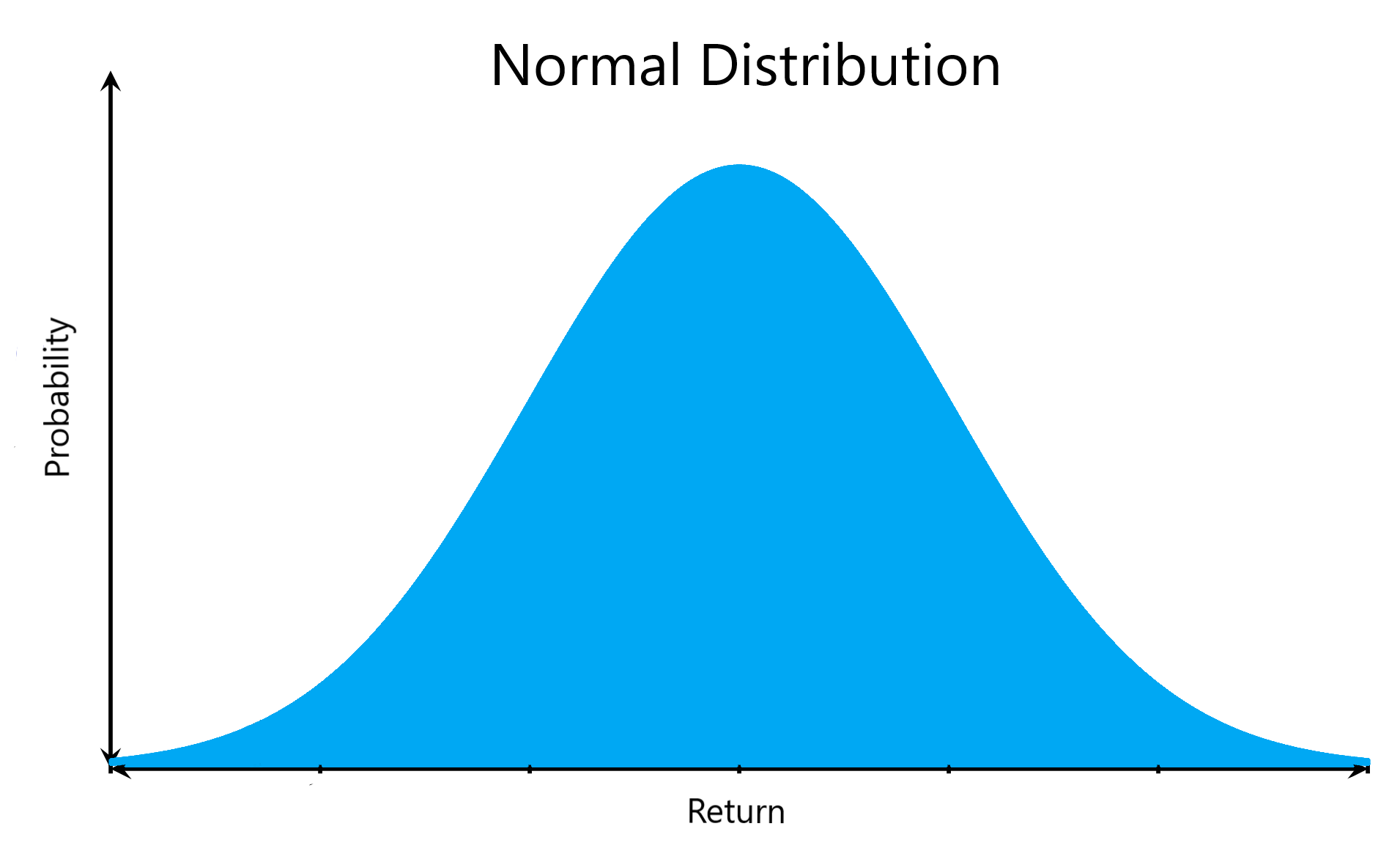
Once we make some assumptions about these factors, we can determine the likelihood of an investment's return in any year. If we assumed investment returns had a distribution shape that was a normal distribution, we could then randomly pick one of the returns within the blue area below for use in our Monte Carlo Analysis.
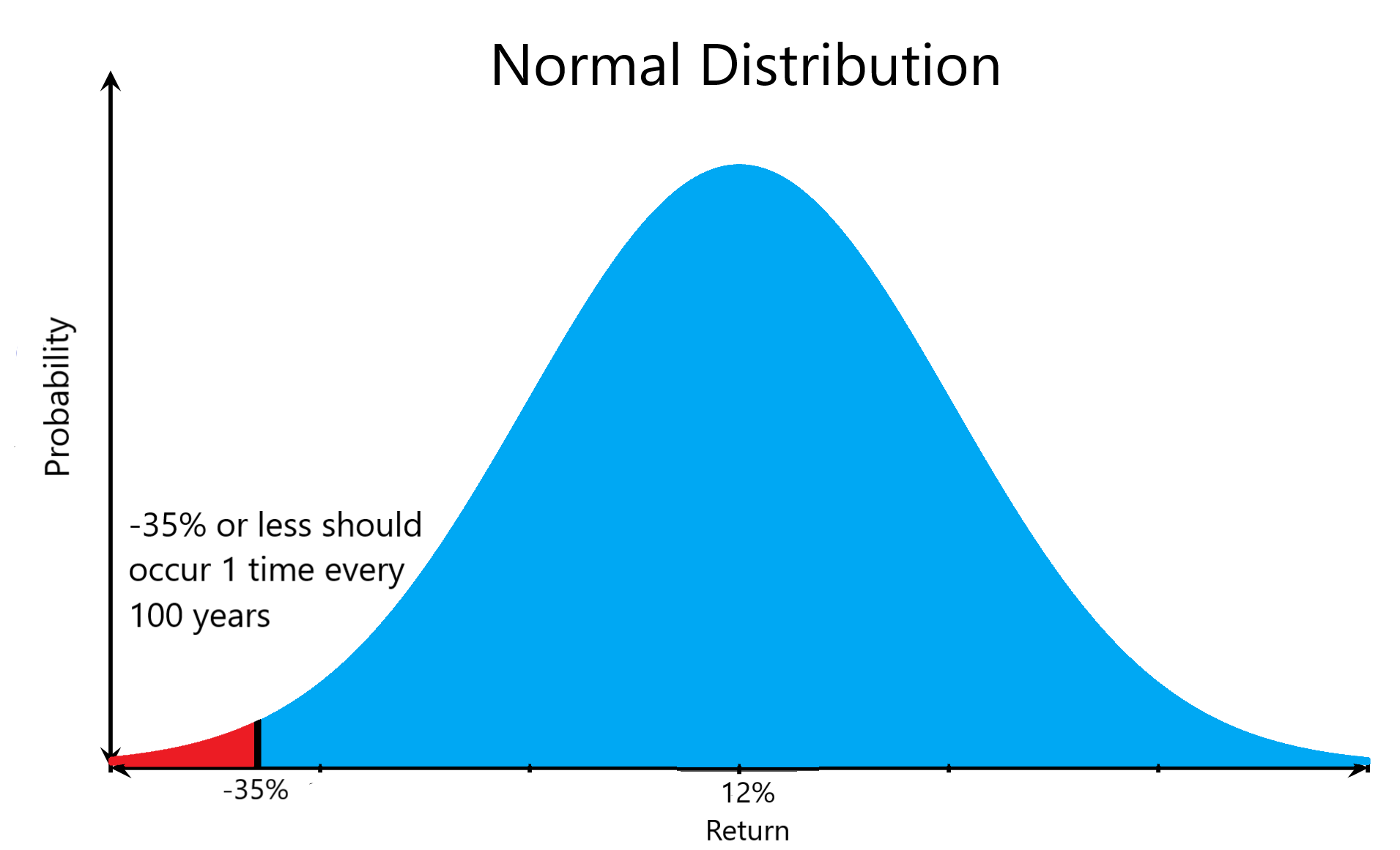
For example, let's assume that the large-cap equity asset category has an arithmetic return of 8% with a 20% standard deviation, and followed a normal distribution. If that were true, then when we picked a random return for our simulation, we know that 12% will be the most likely return chosen and that a return less than or equal to -35% would occur roughly 1 time every 100 years.
However, is a normal distribution a good assumption?
Where Others Fall Short: Normal Distributions
A common problem with most financial planning software is that they assume stock returns follow a normal distribution. As shown above, a normal distribution would assume that the S&P 500 would have a loss of 35% or less roughly 1 time every 100 years. Instead, the S&P 500 has lost 35% or more 3 times in the last 93 years**. As with all financial models, garbage in means garbage out. Financial planning is most concerned with downside scenarios, and assuming investment returns are normally distributed underestimates the risk in your financial plan.
The ComposedPro Difference: Non-Normal Distributions
We do not assume that investment returns follow a normal distribution in our financial plans. Instead, we make the following two adjustments to capture the downside risk exhibited by investment returns:
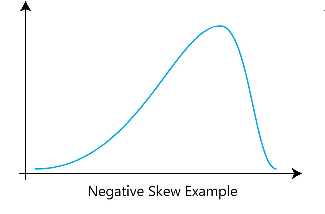
- Skewness - Skewness tilts the peak of the distribution to the left or right. In our previous example using the S&P 500, we would assume a negative skew, meaning the peak of the distribution is tilted to the right. It makes the left tail of the distribution longer, meaning extreme downside scenarios are more likely as compared to a normal distribution.
Disclosures:
ComposedPro makes no warranties, expressed or implied, as to the accuracy, completeness, or results of any of the financial plan calculations generated by its third-party financial planning software. Please read disclosures provided by our third-party financial planning software on the financial plan generated for more information. Adjusting investment return distributions shapes to more accurately represent historical investment returns may not be an accurate representation of future investment returns. Furthermore, historical investment returns are a simplifying assumption used to model future investment returns for illustrative purposes only. In reality, investment returns are highly volatile and past returns are not indicative of future results. Any historical returns discussed in this article or used in the financial plan models created by ComposedPro's third-party financial planning software will not necessarily be accurate going forward. Nothing contained within this email transmission should be relied upon for making any investment decision. Any information provided is for information purposes only and does not constitute a recommendation. Any data in this article or in financial plans generated by ComposedPro's third-party financial planning software that simulate future scenarios are not guaranteed. The inputs provided by clients used to generate financial plan models are key inputs in each financial plan. Such information provided by the user should be periodically reviews and updated when circumstances may require.
Comments
0 comments
Article is closed for comments.